Gaussian process regression in six questions
15 June 2026
Gaussian processes are one of the cleanest tools for regression with uncertainty: a handful of linear algebra, a kernel, and you get a mean prediction together with an honest error bar. This post walks through the questions I find most useful for actually understanding them. It is based on a tutorial I co-wrote for Algorithms for Uncertainty Quantification at TUM, and ends with a short numpy implementation you can run yourself.
1. What is a Gaussian process?
A Gaussian process is a distribution over functions. Any finite set of function values \(f(x_1), \dots, f(x_n)\) is jointly Gaussian, and the whole process is fully specified by two objects:
- a mean function \(m(x)\), our best guess before seeing data (often just zero), and
- a covariance function or kernel \(k(x, x')\), which says how strongly the values at \(x\) and \(x'\) move together.
The kernel carries almost all of the modelling. A common choice is the squared exponential (SE) kernel
\[k_\theta(x, x') = \sigma_f^2 \exp\left(-\frac{(x - x')^2}{2\ell^2}\right),\]where the length scale \(\ell\) sets how far apart two inputs can be and still be correlated, and \(\sigma_f\) sets the overall amplitude of the function.
2. What happens when we observe data?
We usually observe noisy values \(y_i = f(x_i) + \eta_i\) with \(\eta_i \sim \mathcal{N}(0, \sigma_n^2)\). Under the GP prior, the training outputs \(y\) and the unknown function values \(f_*\) at test inputs \(X_*\) are jointly Gaussian:
\[\begin{pmatrix} y \\ f_* \end{pmatrix} \sim \mathcal{N}\left(0, \begin{pmatrix} K(X, X) + \sigma_n^2 I & K(X, X_*) \\ K(X_*, X) & K(X_*, X_*) \end{pmatrix}\right).\]Conditioning a Gaussian on part of its entries gives another Gaussian. Writing \(K_y = K(X, X) + \sigma_n^2 I\), the posterior is
\[\bar f_* = K(X_*, X)\, K_y^{-1} y, \qquad \operatorname{Cov}(f_*) = K(X_*, X_*) - K(X_*, X)\, K_y^{-1} K(X, X_*).\]That is the entire method. Everything else is about computing this stably and choosing the kernel well.
3. Why can data only reduce uncertainty?
Look at the posterior covariance: it is the prior covariance minus the term \(K(X_*, X) K_y^{-1} K(X, X_*)\). Since \(K_y\) is positive definite, so is its inverse, and a matrix of the form \(B^\top A B\) with \(A\) positive definite is positive semi-definite. So the correction never adds variance: at every test point at once, the posterior variance is at most the prior variance. Near the data it drops a lot; far away the correction vanishes and we fall back to the prior.
There is a second, less obvious consequence. The posterior covariance contains no \(y\). For fixed hyperparameters, the uncertainty depends only on where we observed, not on what we observed. The observed values move the mean; the input locations shape the error bars. This is exactly why GPs are so useful for experimental design and active learning: you can decide where to measure next before you know the result.
4. How do I draw sample functions?
To sample \(f \sim \mathcal{N}(\mu, \Sigma)\), factor \(\Sigma = L L^\top\) with a Cholesky decomposition and return \(\mu + L z\) with \(z \sim \mathcal{N}(0, I)\). Then \(\operatorname{Cov}(Lz) = L L^\top = \Sigma\), as required.
You need the full covariance here, not just its diagonal. The off-diagonal entries are what make neighbouring points move together. If you used only the diagonal, each point would get independent noise and your “sample function” would be a jagged cloud with the right pointwise spread but none of the smoothness the kernel encodes.
5. What does the 95% band mean?
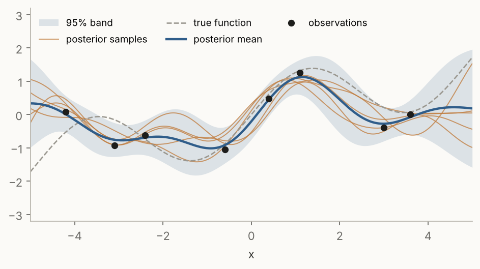
The band \(\bar f_*(x) \pm 1.96 \sqrt{\operatorname{Var}(f_*(x))}\) uses the fact that a standard normal puts 95% of its mass within 1.96 standard deviations of the mean. It is a pointwise statement: at each \(x\) separately, the true value lies in the band with probability 0.95.
That does not mean whole sample paths stay inside. A path crosses many points, and the chance that it stays inside the band at all of them is lower than 95%. In the figure below you can see posterior samples stepping outside the shaded region now and then, which is exactly what should happen.
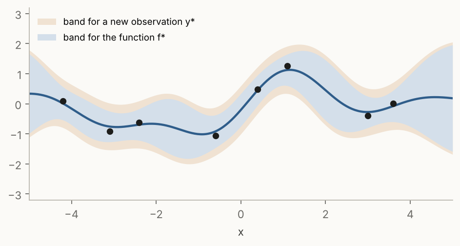
Note also which band you want. The band above is for the latent function \(f_*\). If you want to predict a new noisy measurement \(y_* = f(x_*) + \eta_*\), you add the noise back in: \(\operatorname{Var}(y_* \mid \text{data}) = \operatorname{Var}(f_* \mid \text{data}) + \sigma_n^2\). Use the first to say where the function is, the second to say where the next data point will land.
6. How do I choose the hyperparameters?
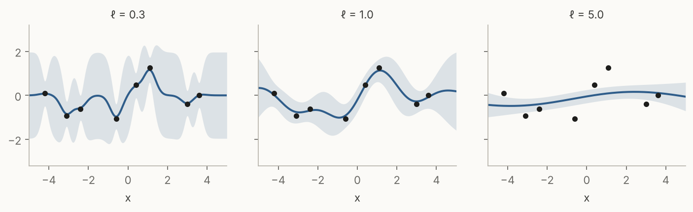
The kernel hyperparameters \(\theta = (\ell, \sigma_f, \sigma_n)\) matter a lot. With a short length scale, the mean chases every data point and snaps back to the prior in between. With a long one, it smooths through the data and ignores real structure.
The standard way to pick them is to maximise the log marginal likelihood:
\[\log p(y \mid X, \theta) = \underbrace{-\tfrac{1}{2} y^\top K_y^{-1} y}_{\text{data fit}} \;\underbrace{-\tfrac{1}{2} \log \det K_y}_{\text{complexity}} \;\underbrace{-\tfrac{n}{2} \log 2\pi}_{\text{constant}}.\]The data fit term rewards explaining the observations. The complexity term penalises flexible models: a short length scale makes the kernel matrix close to diagonal, which pushes \(\det K_y\) up and the penalty with it. The constant does not depend on \(\theta\). Maximising the sum is a built-in Occam’s razor: the preferred model is the simplest one that still explains the data, without any separate validation set.
Implementation in numpy
Here is the whole thing in about twenty lines. It never forms an explicit inverse: a Cholesky factorisation and two triangular solves are faster and numerically much more stable.
import numpy as np

def se_kernel(a, b, ell=1.0, sf=1.0):
    return sf**2 * np.exp(-0.5 * (a[:, None] - b[None, :])**2 / ell**2)

def gp_posterior(X, y, Xs, ell=1.0, sf=1.0, sn=0.3):
    Ky = se_kernel(X, X, ell, sf) + sn**2 * np.eye(len(X))
    L = np.linalg.cholesky(Ky)                   # Ky = L L^T
    alpha = np.linalg.solve(L.T, np.linalg.solve(L, y))
    Ks = se_kernel(Xs, X, ell, sf)
    mean = Ks @ alpha
    V = np.linalg.solve(L, Ks.T)
    cov = se_kernel(Xs, Xs, ell, sf) - V.T @ V
    return mean, cov

def sample_paths(mean, cov, n=5, jitter=1e-8, rng=np.random.default_rng(0)):
    Lp = np.linalg.cholesky(cov + jitter * np.eye(len(mean)))
    return mean[:, None] + Lp @ rng.standard_normal((len(mean), n))
The small jitter on the diagonal keeps the Cholesky factorisation stable: posterior covariances are often positive semi-definite only up to rounding error.
Takeaways
- A GP is a distribution over functions, specified by a mean and a kernel.
- Conditioning on data is just conditioning a Gaussian, and it can only reduce variance.
- For fixed hyperparameters, the uncertainty depends on where you measured, not on what you measured.
- Sampling needs the full covariance; the 95% band is pointwise.
- The marginal likelihood balances data fit against complexity and picks hyperparameters without a validation set.