<?xml version="1.0" encoding="utf-8"?><feed xmlns="http://www.w3.org/2005/Atom" xml:lang="en"><generator uri="https://jekyllrb.com/" version="3.10.0">Jekyll</generator><link href="https://ioandanielc.github.io/blog/feed.xml" rel="self" type="application/atom+xml" /><link href="https://ioandanielc.github.io/" rel="alternate" type="text/html" hreflang="en" /><updated>2026-10-09T13:11:24+00:00</updated><id>https://ioandanielc.github.io/blog/feed.xml</id><title type="html">Ioan-Daniel Craciun</title><subtitle>PhD student in scientific machine learning at the Technical University of Munich.</subtitle><author><name>Ioan-Daniel Craciun</name></author><entry><title type="html">Gaussian process regression in six questions</title><link href="https://ioandanielc.github.io/blog/2026/gaussian-process-regression/" rel="alternate" type="text/html" title="Gaussian process regression in six questions" /><published>2026-06-15T00:00:00+00:00</published><updated>2026-06-15T00:00:00+00:00</updated><id>https://ioandanielc.github.io/blog/2026/gaussian-process-regression</id><content type="html" xml:base="https://ioandanielc.github.io/blog/2026/gaussian-process-regression/"><![CDATA[<p>Gaussian processes are one of the cleanest tools for regression with uncertainty: a handful of linear algebra, a kernel, and you get a mean prediction together with an honest error bar. This post walks through the questions I find most useful for actually understanding them. It is based on a tutorial I co-wrote for <em>Algorithms for Uncertainty Quantification</em> at TUM, and ends with a short numpy implementation you can run yourself.</p>

<h2 id="1-what-is-a-gaussian-process">1. What is a Gaussian process?</h2>

<p>A Gaussian process is a distribution over <strong>functions</strong>. Any finite set of function values \(f(x_1), \dots, f(x_n)\) is jointly Gaussian, and the whole process is fully specified by two objects:</p>

<ul>
  <li>a <strong>mean function</strong> \(m(x)\), our best guess before seeing data (often just zero), and</li>
  <li>a <strong>covariance function</strong> or kernel \(k(x, x')\), which says how strongly the values at \(x\) and \(x'\) move together.</li>
</ul>

<p>The kernel carries almost all of the modelling. A common choice is the squared exponential (SE) kernel</p>

\[k_\theta(x, x') = \sigma_f^2 \exp\left(-\frac{(x - x')^2}{2\ell^2}\right),\]

<p>where the length scale \(\ell\) sets how far apart two inputs can be and still be correlated, and \(\sigma_f\) sets the overall amplitude of the function.</p>

<h2 id="2-what-happens-when-we-observe-data">2. What happens when we observe data?</h2>

<p>We usually observe noisy values \(y_i = f(x_i) + \eta_i\) with \(\eta_i \sim \mathcal{N}(0, \sigma_n^2)\). Under the GP prior, the training outputs \(y\) and the unknown function values \(f_*\) at test inputs \(X_*\) are jointly Gaussian:</p>

\[\begin{pmatrix} y \\ f_* \end{pmatrix}
\sim \mathcal{N}\left(0,
\begin{pmatrix} K(X, X) + \sigma_n^2 I &amp; K(X, X_*) \\ K(X_*, X) &amp; K(X_*, X_*) \end{pmatrix}\right).\]

<p>Conditioning a Gaussian on part of its entries gives another Gaussian. Writing \(K_y = K(X, X) + \sigma_n^2 I\), the posterior is</p>

\[\bar f_* = K(X_*, X)\, K_y^{-1} y,
\qquad
\operatorname{Cov}(f_*) = K(X_*, X_*) - K(X_*, X)\, K_y^{-1} K(X, X_*).\]

<p>That is the entire method. Everything else is about computing this stably and choosing the kernel well.</p>

<h2 id="3-why-can-data-only-reduce-uncertainty">3. Why can data only reduce uncertainty?</h2>

<p>Look at the posterior covariance: it is the prior covariance minus the term \(K(X_*, X) K_y^{-1} K(X, X_*)\). Since \(K_y\) is positive definite, so is its inverse, and a matrix of the form \(B^\top A B\) with \(A\) positive definite is positive semi-definite. So the correction never adds variance: at every test point at once, the posterior variance is at most the prior variance. Near the data it drops a lot; far away the correction vanishes and we fall back to the prior.</p>

<p>There is a second, less obvious consequence. The posterior covariance contains <strong>no</strong> \(y\). For fixed hyperparameters, the uncertainty depends only on <em>where</em> we observed, not on <em>what</em> we observed. The observed values move the mean; the input locations shape the error bars. This is exactly why GPs are so useful for experimental design and active learning: you can decide where to measure next before you know the result.</p>

<h2 id="4-how-do-i-draw-sample-functions">4. How do I draw sample functions?</h2>

<p>To sample \(f \sim \mathcal{N}(\mu, \Sigma)\), factor \(\Sigma = L L^\top\) with a Cholesky decomposition and return \(\mu + L z\) with \(z \sim \mathcal{N}(0, I)\). Then \(\operatorname{Cov}(Lz) = L L^\top = \Sigma\), as required.</p>

<p>You need the <strong>full</strong> covariance here, not just its diagonal. The off-diagonal entries are what make neighbouring points move together. If you used only the diagonal, each point would get independent noise and your “sample function” would be a jagged cloud with the right pointwise spread but none of the smoothness the kernel encodes.</p>

<h2 id="5-what-does-the-95-band-mean">5. What does the 95% band mean?</h2>

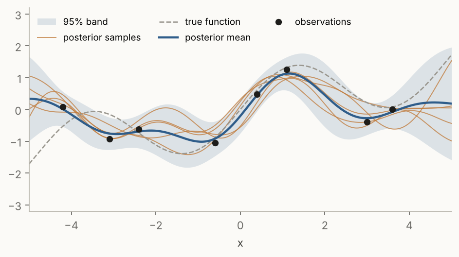
<p>The band \(\bar f_*(x) \pm 1.96 \sqrt{\operatorname{Var}(f_*(x))}\) uses the fact that a standard normal puts 95% of its mass within 1.96 standard deviations of the mean. It is a <strong>pointwise</strong> statement: at each \(x\) separately, the true value lies in the band with probability 0.95.</p>

<p>That does not mean whole sample paths stay inside. A path crosses many points, and the chance that it stays inside the band at all of them is lower than 95%. In the figure below you can see posterior samples stepping outside the shaded region now and then, which is exactly what should happen.</p>

<p><img src="/assets/img/gp-posterior.png" alt="GP posterior with 95% band and five posterior samples" /></p>

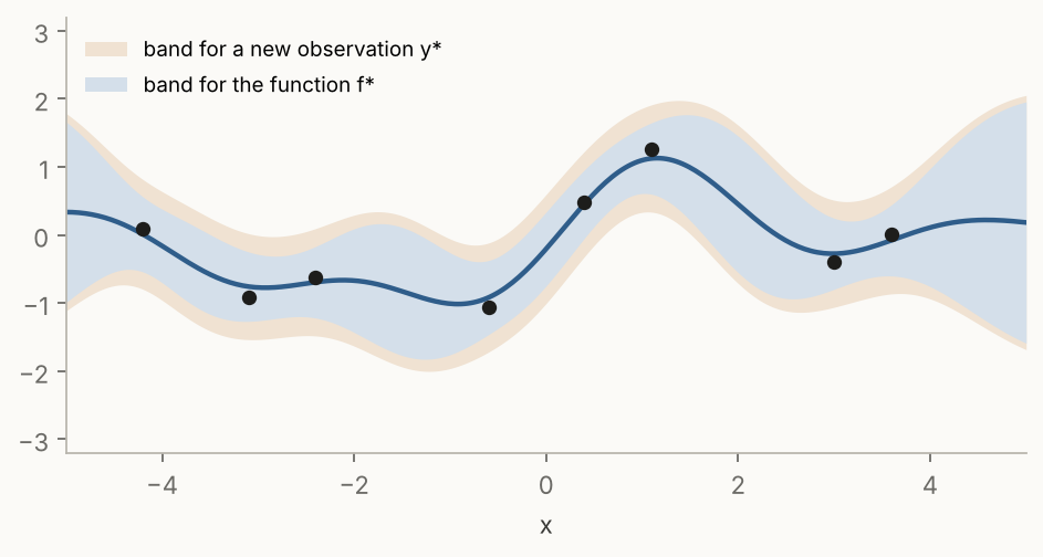
<p>Note also which band you want. The band above is for the latent function \(f_*\). If you want to predict a <strong>new noisy measurement</strong> \(y_* = f(x_*) + \eta_*\), you add the noise back in: \(\operatorname{Var}(y_* \mid \text{data}) = \operatorname{Var}(f_* \mid \text{data}) + \sigma_n^2\). Use the first to say where the function is, the second to say where the next data point will land.</p>

<p><img src="/assets/img/gp-f-vs-y.png" alt="Band for the latent function compared with the band for a new observation" /></p>

<h2 id="6-how-do-i-choose-the-hyperparameters">6. How do I choose the hyperparameters?</h2>

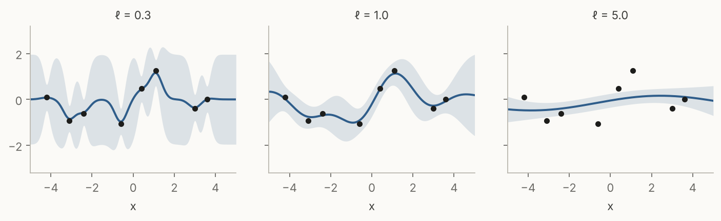
<p>The kernel hyperparameters \(\theta = (\ell, \sigma_f, \sigma_n)\) matter a lot. With a short length scale, the mean chases every data point and snaps back to the prior in between. With a long one, it smooths through the data and ignores real structure.</p>

<p><img src="/assets/img/gp-lengthscales.png" alt="Posterior for length scales 0.3, 1.0 and 5.0" /></p>

<p>The standard way to pick them is to maximise the log marginal likelihood:</p>

\[\log p(y \mid X, \theta)
= \underbrace{-\tfrac{1}{2} y^\top K_y^{-1} y}_{\text{data fit}}
\;\underbrace{-\tfrac{1}{2} \log \det K_y}_{\text{complexity}}
\;\underbrace{-\tfrac{n}{2} \log 2\pi}_{\text{constant}}.\]

<p>The <strong>data fit</strong> term rewards explaining the observations. The <strong>complexity</strong> term penalises flexible models: a short length scale makes the kernel matrix close to diagonal, which pushes \(\det K_y\) up and the penalty with it. The constant does not depend on \(\theta\). Maximising the sum is a built-in Occam’s razor: the preferred model is the simplest one that still explains the data, without any separate validation set.</p>

<h2 id="implementation-in-numpy">Implementation in numpy</h2>

<p>Here is the whole thing in about twenty lines. It never forms an explicit inverse: a Cholesky factorisation and two triangular solves are faster and numerically much more stable.</p>

<div class="language-python highlighter-rouge"><div class="highlight"><pre class="highlight"><code><span class="kn">import</span> <span class="nn">numpy</span> <span class="k">as</span> <span class="n">np</span>

<span class="k">def</span> <span class="nf">se_kernel</span><span class="p">(</span><span class="n">a</span><span class="p">,</span> <span class="n">b</span><span class="p">,</span> <span class="n">ell</span><span class="o">=</span><span class="mf">1.0</span><span class="p">,</span> <span class="n">sf</span><span class="o">=</span><span class="mf">1.0</span><span class="p">):</span>
    <span class="k">return</span> <span class="n">sf</span><span class="o">**</span><span class="mi">2</span> <span class="o">*</span> <span class="n">np</span><span class="p">.</span><span class="n">exp</span><span class="p">(</span><span class="o">-</span><span class="mf">0.5</span> <span class="o">*</span> <span class="p">(</span><span class="n">a</span><span class="p">[:,</span> <span class="bp">None</span><span class="p">]</span> <span class="o">-</span> <span class="n">b</span><span class="p">[</span><span class="bp">None</span><span class="p">,</span> <span class="p">:])</span><span class="o">**</span><span class="mi">2</span> <span class="o">/</span> <span class="n">ell</span><span class="o">**</span><span class="mi">2</span><span class="p">)</span>

<span class="k">def</span> <span class="nf">gp_posterior</span><span class="p">(</span><span class="n">X</span><span class="p">,</span> <span class="n">y</span><span class="p">,</span> <span class="n">Xs</span><span class="p">,</span> <span class="n">ell</span><span class="o">=</span><span class="mf">1.0</span><span class="p">,</span> <span class="n">sf</span><span class="o">=</span><span class="mf">1.0</span><span class="p">,</span> <span class="n">sn</span><span class="o">=</span><span class="mf">0.3</span><span class="p">):</span>
    <span class="n">Ky</span> <span class="o">=</span> <span class="n">se_kernel</span><span class="p">(</span><span class="n">X</span><span class="p">,</span> <span class="n">X</span><span class="p">,</span> <span class="n">ell</span><span class="p">,</span> <span class="n">sf</span><span class="p">)</span> <span class="o">+</span> <span class="n">sn</span><span class="o">**</span><span class="mi">2</span> <span class="o">*</span> <span class="n">np</span><span class="p">.</span><span class="n">eye</span><span class="p">(</span><span class="nb">len</span><span class="p">(</span><span class="n">X</span><span class="p">))</span>
    <span class="n">L</span> <span class="o">=</span> <span class="n">np</span><span class="p">.</span><span class="n">linalg</span><span class="p">.</span><span class="n">cholesky</span><span class="p">(</span><span class="n">Ky</span><span class="p">)</span>                   <span class="c1"># Ky = L L^T
</span>    <span class="n">alpha</span> <span class="o">=</span> <span class="n">np</span><span class="p">.</span><span class="n">linalg</span><span class="p">.</span><span class="n">solve</span><span class="p">(</span><span class="n">L</span><span class="p">.</span><span class="n">T</span><span class="p">,</span> <span class="n">np</span><span class="p">.</span><span class="n">linalg</span><span class="p">.</span><span class="n">solve</span><span class="p">(</span><span class="n">L</span><span class="p">,</span> <span class="n">y</span><span class="p">))</span>
    <span class="n">Ks</span> <span class="o">=</span> <span class="n">se_kernel</span><span class="p">(</span><span class="n">Xs</span><span class="p">,</span> <span class="n">X</span><span class="p">,</span> <span class="n">ell</span><span class="p">,</span> <span class="n">sf</span><span class="p">)</span>
    <span class="n">mean</span> <span class="o">=</span> <span class="n">Ks</span> <span class="o">@</span> <span class="n">alpha</span>
    <span class="n">V</span> <span class="o">=</span> <span class="n">np</span><span class="p">.</span><span class="n">linalg</span><span class="p">.</span><span class="n">solve</span><span class="p">(</span><span class="n">L</span><span class="p">,</span> <span class="n">Ks</span><span class="p">.</span><span class="n">T</span><span class="p">)</span>
    <span class="n">cov</span> <span class="o">=</span> <span class="n">se_kernel</span><span class="p">(</span><span class="n">Xs</span><span class="p">,</span> <span class="n">Xs</span><span class="p">,</span> <span class="n">ell</span><span class="p">,</span> <span class="n">sf</span><span class="p">)</span> <span class="o">-</span> <span class="n">V</span><span class="p">.</span><span class="n">T</span> <span class="o">@</span> <span class="n">V</span>
    <span class="k">return</span> <span class="n">mean</span><span class="p">,</span> <span class="n">cov</span>

<span class="k">def</span> <span class="nf">sample_paths</span><span class="p">(</span><span class="n">mean</span><span class="p">,</span> <span class="n">cov</span><span class="p">,</span> <span class="n">n</span><span class="o">=</span><span class="mi">5</span><span class="p">,</span> <span class="n">jitter</span><span class="o">=</span><span class="mf">1e-8</span><span class="p">,</span> <span class="n">rng</span><span class="o">=</span><span class="n">np</span><span class="p">.</span><span class="n">random</span><span class="p">.</span><span class="n">default_rng</span><span class="p">(</span><span class="mi">0</span><span class="p">)):</span>
    <span class="n">Lp</span> <span class="o">=</span> <span class="n">np</span><span class="p">.</span><span class="n">linalg</span><span class="p">.</span><span class="n">cholesky</span><span class="p">(</span><span class="n">cov</span> <span class="o">+</span> <span class="n">jitter</span> <span class="o">*</span> <span class="n">np</span><span class="p">.</span><span class="n">eye</span><span class="p">(</span><span class="nb">len</span><span class="p">(</span><span class="n">mean</span><span class="p">)))</span>
    <span class="k">return</span> <span class="n">mean</span><span class="p">[:,</span> <span class="bp">None</span><span class="p">]</span> <span class="o">+</span> <span class="n">Lp</span> <span class="o">@</span> <span class="n">rng</span><span class="p">.</span><span class="n">standard_normal</span><span class="p">((</span><span class="nb">len</span><span class="p">(</span><span class="n">mean</span><span class="p">),</span> <span class="n">n</span><span class="p">))</span>
</code></pre></div></div>

<p>The small <code class="language-plaintext highlighter-rouge">jitter</code> on the diagonal keeps the Cholesky factorisation stable: posterior covariances are often positive semi-definite only up to rounding error.</p>

<h2 id="takeaways">Takeaways</h2>

<ul>
  <li>A GP is a distribution over functions, specified by a mean and a kernel.</li>
  <li>Conditioning on data is just conditioning a Gaussian, and it can only reduce variance.</li>
  <li>For fixed hyperparameters, the uncertainty depends on where you measured, not on what you measured.</li>
  <li>Sampling needs the full covariance; the 95% band is pointwise.</li>
  <li>The marginal likelihood balances data fit against complexity and picks hyperparameters without a validation set.</li>
</ul>]]></content><author><name>Ioan-Daniel Craciun</name></author><summary type="html"><![CDATA[Gaussian processes are one of the cleanest tools for regression with uncertainty: a handful of linear algebra, a kernel, and you get a mean prediction together with an honest error bar. This post walks through the questions I find most useful for actually understanding them. It is based on a tutorial I co-wrote for Algorithms for Uncertainty Quantification at TUM, and ends with a short numpy implementation you can run yourself.]]></summary></entry></feed>